A Guide to Cluster Analysis in R

Author

Jason Gavrilis

Introduction

Cluster analysis is a common statistical technique used in many fields such as marketing, healthcare (Loftus et al. 2022), and sports science (Anıl Duman, Sennaroğlu, and Tuzkaya 2021).

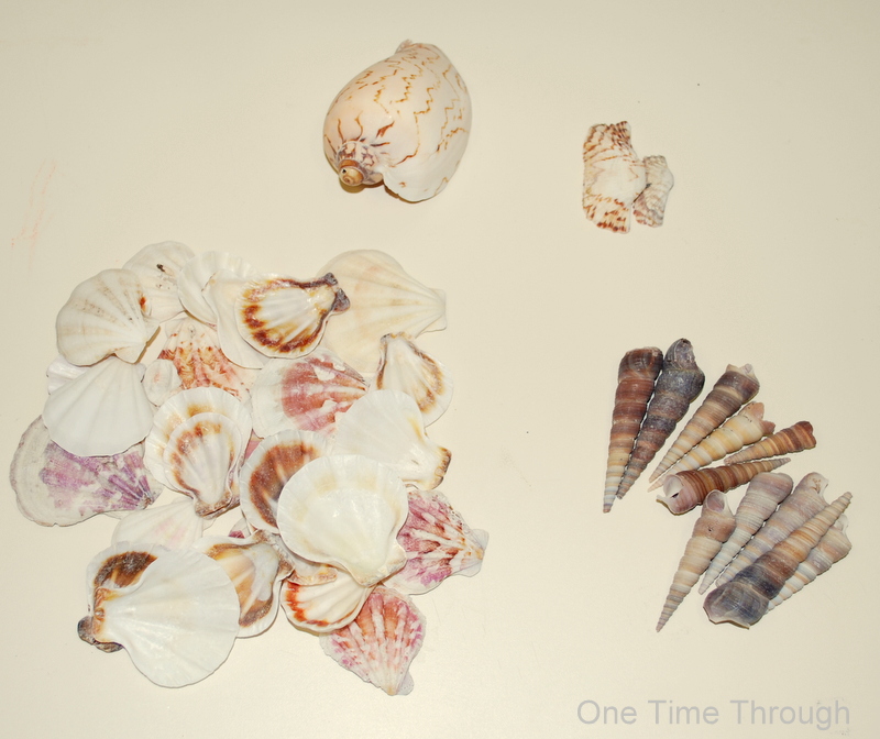
At its core, cluster analysis is a mathematical method for processing data, organizing items into groups or clusters based on how closely associated they are. For example, if you gathered shells from the beach, noted their attributes of size, shape, colour, and sorted similar shells into piles, you would be performing a ‘physical’ cluster analysis. Each pile of shells would be a ‘cluster’ (Romesburg 2004).

Sorting shells into clusters based on physical characteristics (e.g. shape)

Instead of physically sorting objects, a mathematical cluster analysis sorts objects described as data, whereby similar digital descriptions of the objects are mathematically gathered into the same cluster (Romesburg 2004).

The following article steps through a cluster analysis example in R using the banknote data set and the mclust package.

Prerequisites

Load required packages:

Code

if (!require(pacman)) install.packages("pacman")
library(pacman)
p_load(
  tidyverse, gt, mclust, ggpubr, factoextra
)

Data

The banknote data set contains six measurements made on 100 genuine and 100 counterfeit old-Swiss 1000-franc bank notes.

Importantly, there is a variable in the data set called status which groups the banknotes into either genuine or counterfeit:

Code

banknote %>%
  arrange(Length) %>%
  head(5) %>%
  gt::gt() %>%
  gt::tab_options(
    column_labels.font.weight = "bold",
    table.width = pct(80)
  )

Status	Length	Left	Right	Bottom	Top	Diagonal
genuine	213.8	129.8	129.5	8.4	11.1	140.9
genuine	213.9	130.3	129.0	8.1	9.7	141.3
counterfeit	213.9	130.7	130.5	8.7	11.5	137.8
genuine	214.1	129.6	129.3	7.6	10.7	141.7
counterfeit	214.2	130.0	130.2	11.0	11.2	139.5

Here is a summary of the banknote data:

Code

banknote_names <-
  names(banknote %>% select(-Status))

box_plot <- function(df, yvar, fill_var, ...) {
  plot <-
    df %>%
    ggpubr::ggboxplot(
      y = yvar,
      fill = fill_var
    ) +
    scale_fill_manual(values = c("#E64B35", "white")) +
    theme(
      axis.ticks = element_blank(),
      axis.text.x = element_blank(),
      axis.title.x = element_blank()
    )

  return(plot)
}


plot_list <-
  purrr::map(banknote_names, ~ box_plot(banknote, yvar = ., fill_var = "Status"))

original_plot <-
  patchwork::wrap_plots(plot_list) +
    patchwork::plot_layout(guides = "collect") &
    theme(legend.position = "top")

original_plot

For certain measurements, such as the diagonal, there is a clear difference between genuine and counterfeit banknotes. However, for other measurements, like length, the difference is not as obvious. In a scenario where the status of the banknotes is unknown, cluster analysis can be employed to classify the banknotes as real or fake based on the six available measurement.

Cluster Analysis with mclust

mclust is an R package for model-based clustering, classification, and density estimation based on finite Gaussian mixture modelling (Scrucca et al. 2016).

Let’s use mclust to run cluster analysis on the banknote data set (with the status variable removed).

First we create the model with the Mclust function:

Code

note <-
  banknote %>%
  select(-Status)

mod1 <-
  mclust::Mclust(note, verbose = F)

Next we look at the model selection:

Code

factoextra::fviz_mclust(mod1, "BIC", palette = "npg")

As you can see the winning model based on Bayesian Information Criterion (BIC) is the VVE model with three clusters (red vertical dotted line). Thus, the Mclust function automatically performed the analysis based on three clusters.

The cluster plot shows how each banknote was clustered:

Code

factoextra::fviz_mclust(mod1, "classification", palette = "npg")

Let’s take at look at how the model performed based on the known banknote status:

Code

table(banknote$Status, mod1$classification)

             
               1  2  3
  counterfeit 16  0 84
  genuine      2 98  0

The model performed well in identifying genuine banknotes by grouping the majority of them into cluster 2. However, the counterfeit notes were distributed across two clusters, with 16 notes in cluster 1 and 84 notes in cluster 3. This outcome is sub-optimal, given that we know that there are only two types of banknotes.

It is important to stress that the selected model, based on BIC, may not always be the most optimal. With prior knowledge, the cluster analysis can be constrained to focus on a specific number of clusters. In this case, the prior knowledge that banknotes can only be genuine or fake necessitates the creation of a model with two clusters.

Let’s tweak our model parameters to force the banknotes to be grouped into two-clusters and plot the results:

Code

mod2 <-
  mclust::Mclust(note, G = 2, verbose = F)

factoextra::fviz_mclust(mod2, "classification", palette = "npg")

Now let’s check how this model perform based on the known banknote status:

Code

table(banknote$Status, mod2$classification)

             
                1   2
  counterfeit 100   0
  genuine       1  99

Incredibly, the two cluster model has almost perfectly predicted the original known status of banknotes, with only one incorrect classification!

We can double check the results by plotting the data based on the cluster analysis model and compare it to the original data:

Code

note_with_cluster <-
  cbind(Cluster = mod2$classification, note) %>%
  as_tibble() %>%
  mutate(Cluster = ifelse(Cluster == 2, "genuine", "counterfeit"))

plot_list_cluster <-
  purrr::map(banknote_names, ~ box_plot(note_with_cluster, yvar = ., fill_var = "Cluster"))

model_plot <-
  patchwork::wrap_plots(plot_list_cluster) +
    patchwork::plot_annotation(title = "Model Data") +
    patchwork::plot_layout(guides = "collect", ) &
    theme(legend.position = "top")

model_plot

Code

original_plot +
  patchwork::plot_annotation(title = "Original Data")

As expected, the model data is almost identical to the original!

Final Thoughts

Cluster analysis is a powerful technique for uncovering insights from data by grouping similar observations. The banknote data set serves as a practical example of how cluster analysis can be applied to distinguish between genuine and counterfeit notes. The insights gained from this analysis demonstrate the potential of cluster analysis in real-world applications.

When performing cluster analysis, it is important to consider modeling different numbers of clusters, not just the most optimal based on BIC. Additionally, prior knowledge can be valuable when determining the optimal number of clusters.

References

Anıl Duman, Eyüp, Bahar Sennaroğlu, and Gülfem Tuzkaya. 2021. “A Cluster Analysis of Basketball Players for Each of the Five Traditionally Defined Positions.” Proceedings of the Institution of Mechanical Engineers, Part P: Journal of Sports Engineering and Technology, December, 175433712110620. https://doi.org/10.1177/17543371211062064.

Loftus, Tyler J., Benjamin Shickel, Jeremy A. Balch, Patrick J. Tighe, Kenneth L. Abbott, Brian Fazzone, Erik M. Anderson, et al. 2022. “Phenotype Clustering in Health Care: A Narrative Review for Clinicians.” Frontiers in Artificial Intelligence 5 (August). https://doi.org/10.3389/frai.2022.842306.

Romesburg, Charles. 2004. Cluster Analysis for Researchers. Lulu.com.

Scrucca, Luca, Michael Fop, T. Brendan Murphy, and Adrian E. Raftery. 2016. “Mclust 5: Clustering, Classification and Density Estimation Using gaussian Finite Mixture Models” 8. https://doi.org/10.32614/RJ-2016-021.